Rents in the Bay Area
Loading the data
# download directly off tidytuesdaygithub repo

rent <- readr::read_csv('https://raw.githubusercontent.com/rfordatascience/tidytuesday/master/data/2022/2022-07-05/rent.csv', show_col_types = FALSE)
Ranking of Classifieds - top 20 cities
df_top_twenty <-
  rent %>%
    count(city) %>% #to count number of classifieds in each city
    arrange(desc(n)) %>% #arrange by highest number
    slice(1:20) %>%
    mutate(percentage = n/sum(n))
ggplot(df_top_twenty, aes(x = percentage, y = fct_reorder(city, percentage))) +
  geom_col() +
  theme_bw() +
  labs(
    title = "San Francisco accounts for more than a quarter of all rental classifieds",
    subtitle = "% of Craigslist listings, 2000-2018",
    x = "Rental Classifieds Percentage",
    y = "City",
    caption = "Source: Pennington. Kate (2018). Bay Area Craigslist Rental Housing Posts 2000-2018") +
  scale_x_continuous(labels = scales::percent)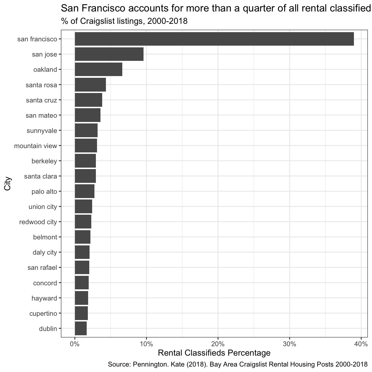
Rentals evolution in San Francisco
#to find the median prices of each each year in San Fancisco
medianPrices <- rent %>%
    filter(city == "san francisco", beds <= 3) %>%
    group_by(beds, year) %>%
    summarize(medianYear = median(price))

ggplot(medianPrices, aes(year, medianYear, color = factor(beds))) +
  geom_line() +
  facet_wrap(vars(beds), nrow = 1) +
  theme_bw() +
  labs(
    title = "San Francisco rentals have been steadily increasing",
    subtitle = "0 to 3-bed listings, 2000-2018",
     x = "Year",
    y = "Rental Price",
    caption = "Source: Pennington. Kate (2018). Bay Area Craigslist Rental Housing Posts 2000-2018") +
  theme(legend.position = "None")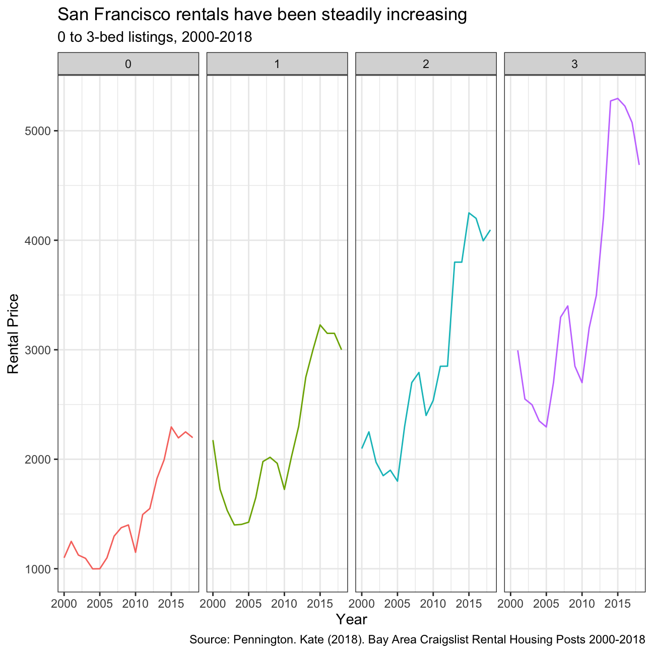
Rentals Evolution in the top 12 cities
#to find the top 12 cities
top_twelve_data <- rent %>%
  count(city) %>% #to count number of classifieds in each city
  arrange(desc(n)) %>%
  slice(1:12)
top_twelve_cities <- as.vector(top_twelve_data$city)
#top_twelve_cities

#Finding median price of each year in the top 12 cities
rent %>%
  filter(city %in% top_twelve_cities) %>%
  group_by(year, city) %>%
  summarize(median_price = median(price)) %>%
ggplot(aes(year, median_price, color = factor(city))) +
  geom_line() +
  facet_wrap(vars(city)) +
  labs(
  title = "Rental prices for flats in the Bay Area",
  x = "Year",
  y = "Rental Price",
  caption = "Source: Pennington. Kate (2018). Bay Area Craigslist Rental Housing Posts 2000-2018") +
  theme(legend.position = "None")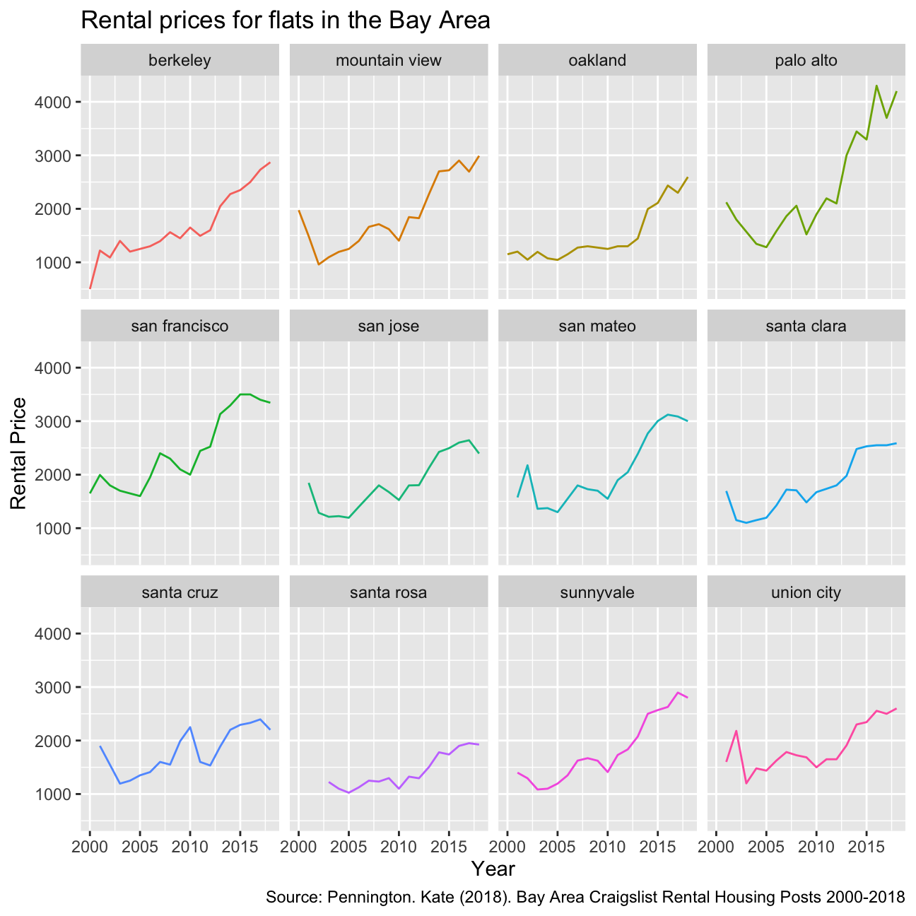
Conclusion
There has been a overall increase in rental prices in the Bay Area between 2000 and 2018. This reflects the tech boom in the Bay Area. In particular, Palo Alto, the birthplace of Sillicon Valley, has experienced the highest rental increase. On the other hand, cities like Santa Rosa and San Jose, have experienced relatively lower rental increase. This increase can probably be accounted for by simple inflation adjustments. Most cities experienced a dip in prices around 2008-2010. We believe this reflects the housing bubble burst of 2008, which triggered a global financial crisis. Before this graphs can be seen to be increasing to a local peak when cheap credit and tax lending standards fueled the housing bubble. After 2010, the government bailouts helped the market recover and restart the economy, giving us an increasing trend in housing prices.