Anomalies in Weather Patterns

Reading the data
weather <-
  read_csv("https://data.giss.nasa.gov/gistemp/tabledata_v4/NH.Ts+dSST.csv",
           skip = 1,
           na = "***")
Plotting the Information
#to select year and 12 months
year_months <- weather %>%
  select(1:13)
#year_months

#converting to long format
tidyweather <- year_months %>%
  pivot_longer(2:13, names_to = "Month", values_to = "delta")
#tidyweather
Weather anomalies for each month
tidyweather <- tidyweather %>%
  mutate(date = ymd(paste(as.character(Year), Month, "1")),
         month = month(date, label=TRUE),
         year = year(date))
tidyweather
## # A tibble: 1,716 × 6
## Year Month delta date month year
## <dbl> <chr> <dbl> <date> <ord> <dbl>
## 1 1880 Jan -0.39 1880-01-01 Jan 1880
## 2 1880 Feb -0.53 1880-02-01 Feb 1880
## 3 1880 Mar -0.23 1880-03-01 Mar 1880
## 4 1880 Apr -0.3 1880-04-01 Apr 1880
## 5 1880 May -0.05 1880-05-01 May 1880
## 6 1880 Jun -0.18 1880-06-01 Jun 1880
## 7 1880 Jul -0.21 1880-07-01 Jul 1880
## 8 1880 Aug -0.25 1880-08-01 Aug 1880
## 9 1880 Sep -0.24 1880-09-01 Sep 1880
## 10 1880 Oct -0.3 1880-10-01 Oct 1880
## # … with 1,706 more rowsg <- ggplot(tidyweather, aes(x=date, y = delta))+
geom_point()+
geom_smooth(color="red") +
theme_bw() +
labs (
title = "Weather Anomalies"
) + facet_wrap(vars(month(date, label=TRUE)))
g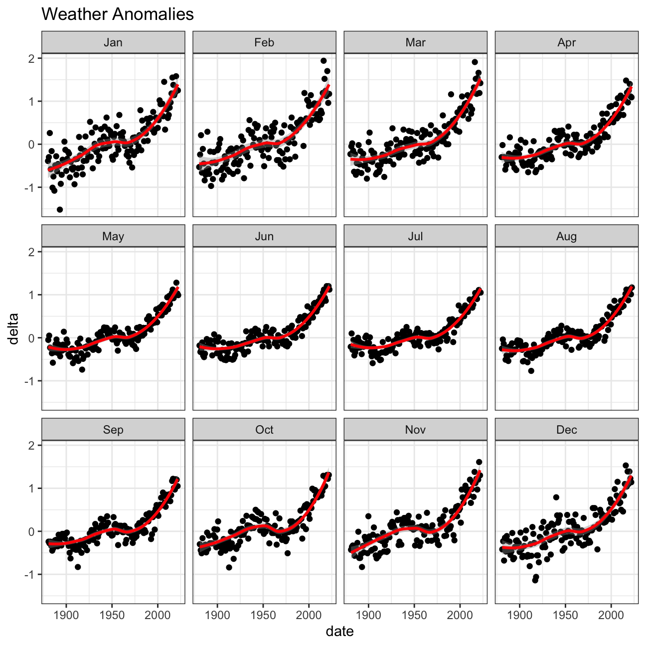
Weather anomalies have an increasing trend, with a steap increase after 1975. The effect of increasing temperature is slightly more pronounced in November.
Weather anomalies for different time periods
Grouping data in five time periods:
comparison <- tidyweather %>%
  filter(Year>= 1881) %>%     #remove years prior to 1881
  #create new variable 'interval', and assign values based on criteria below:
  mutate(interval = case_when(
    Year %in% c(1881:1920) ~ "1881-1920",
    Year %in% c(1921:1950) ~ "1921-1950",
    Year %in% c(1951:1980) ~ "1951-1980",
    Year %in% c(1981:2010) ~ "1981-2010",
    TRUE ~ "2011-present"
  ))
The distribution of monthly deviations (delta), grouped by the different time periods:
g <- ggplot(comparison, aes(delta, fill = interval)) +
  geom_density()
g